
How a neural network learns, from weights to backpropagation
A neural network learns by shrinking its own error, one small step at a time
A neural network learns by making a guess, measuring how wrong the guess was, and nudging thousands or billions of numbers called weights so the next guess is a little less wrong. Gradient descent decides which way to nudge each weight, backpropagation works out how much each weight contributed to the error, and that loop, repeated over many examples, is the whole of training.
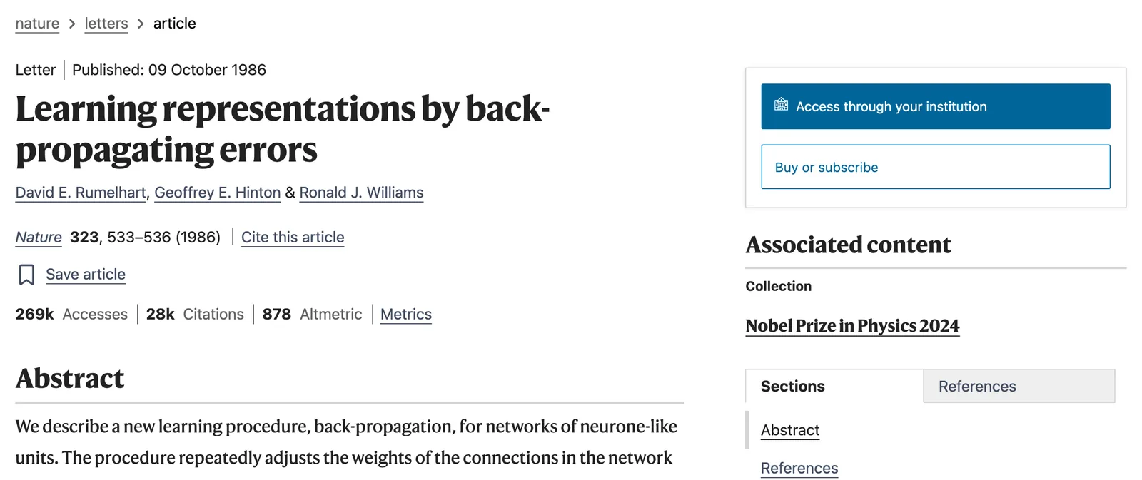
Nothing in that loop is mysterious, and none of it is new. The method that made it practical for networks with hidden layers was published in Nature in October 1986 by David Rumelhart, Geoffrey Hinton and Ronald Williams, and their abstract describes it in one sentence: the procedure “repeatedly adjusts the weights of the connections in the network so as to minimize a measure of the difference between the actual output vector of the net and the desired output vector”. The rest of this post walks through the parts that sentence assumes: the layers, the weights, the loss, gradient descent and backpropagation itself.
If you want to see how this maps onto the models people use at work, the companion explainer on how large language models differ picks up where this one stops, and the rest of the AI explained series covers retrieval and agents.
If you are deciding where AI fits in your business today, a short call will separate what is ready from what is not. Book a call with GenovaFlow AI
Layers are rows of small weighted sums, and the weights are what gets learned
A network is built in layers. The input layer holds the numbers you feed in (pixel values, word tokens turned into numbers, columns from a spreadsheet), the output layer holds the answer, and everything in between is a hidden layer. Google's Machine Learning Crash Course puts it plainly: the additional layers between the input layer and the output layer are called hidden layers, and each neuron in them is computed like a small linear model, with its own weight for every input plus a bias.
The weights and biases are the parameters, and they are the only thing training changes. The same course page counts them for a toy network with three inputs, one hidden layer of four neurons and one output, and arrives at 21 parameters in total. A modern language model has the same kind of parameters, just vastly more of them, which is why the word “parameters” shows up in every model announcement.
Here is one neuron worked through by hand, as an example with made up numbers. It receives two inputs, multiplies each by its weight, adds the bias, then passes the result through an activation function, here ReLU, which returns zero for anything negative.
inputs:      x1 = 2.0, x2 = 1.0
weights:     w1 = 0.5, w2 = -1.5
bias:        b  = 0.25
weighted sum = (2.0 * 0.5) + (1.0 * -1.5) + 0.25 = -0.25
ReLU(-0.25)  = max(0, -0.25) = 0
That activation step matters more than it looks. Google's page on activation functions explains why: linear operations stacked on linear operations are still linear, so without a nonlinear function such as ReLU, sigmoid or tanh between layers, a deep network could only ever draw straight lines through the data, however many layers you gave it.
Gradient descent turns a measured error into a direction to move
Training needs a single number that says how wrong the network is, called the loss. For a price prediction it might be the average squared gap between predicted and real prices; for a classifier it measures how much probability the network put on the wrong label. Once you have that number, the job becomes finding the weights that make it as small as possible.
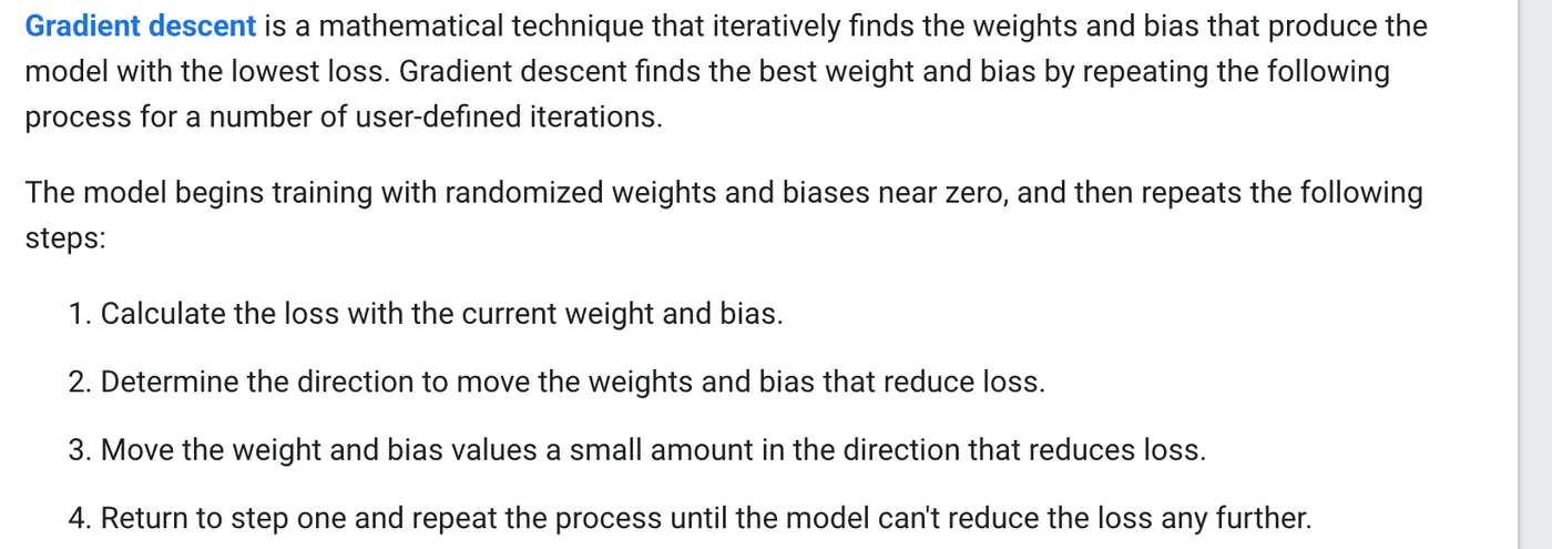
Gradient descent is the search method. In Google's description, the model starts with random weights near zero and then repeats four steps: calculate the loss, work out which direction to move the weights to reduce it, move them a small amount in that direction, and go again until the loss stops falling.
The “small amount” is the learning rate, and it is the setting people tune first. Too large and the weights overshoot the low point and bounce around; too small and training crawls. Real training runs rarely compute the loss over the whole dataset at once. They use small batches of examples per step, which is noisier but far cheaper, and the noise often helps the search avoid getting stuck.
Backpropagation tells every weight how much of the error was its fault
Gradient descent needs a slope for every single weight, and that is the part backpropagation solves. Google's course calls it the most common training algorithm for neural networks, the method that makes gradient descent feasible for networks with several layers. It runs the network forward to get a prediction and a loss, then walks backwards from the output, using the chain rule from calculus to pass the error signal through each layer and give every weight its share of the blame.
The 1986 paper's real contribution was what this did to the hidden layers. Its abstract reports that, as a result of the weight adjustments, the hidden units “come to represent important features of the task domain”. Nobody tells the network which features to look for; the features appear because they help reduce the loss.
That idea earned formal recognition decades later. On 8 October 2024 the Royal Swedish Academy of Sciences awarded the Nobel Prize in Physics to John Hopfield and Geoffrey Hinton “for foundational discoveries and inventions that enable machine learning with artificial neural networks”.
Backpropagation has known failure modes, and the same course page lists them. Gradients can shrink towards zero in the lower layers so those layers barely train (vanishing gradients), grow too large to converge (exploding gradients), or leave a ReLU unit stuck at zero for good. The standard fixes are choices you will see in any training script: ReLU activations, batch normalisation, a lower learning rate, and dropout, which randomly switches off units for a single training step to stop the network memorising its training data.
The same loop trains image models and language models today
What changed after 1986 was scale, data and architecture, not the learning rule. The image network from Krizhevsky, Sutskever and Hinton at NeurIPS 2012 was trained on 1.3 million images in 1,000 classes and had 60 million parameters and 500,000 neurons across five convolutional layers, still trained with gradient descent and backpropagation.
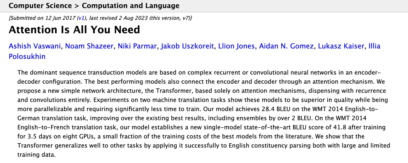
The architecture behind today's language models came in June 2017. The transformer paper, Attention Is All You Need, replaced the recurrent and convolutional layers used for translation with attention, a mechanism that lets every word weigh every other word in the input. The paper reports 28.4 BLEU on English to German translation and 41.8 on English to French after training for 3.5 days on eight GPUs. Inside, it is still layers of weights, a loss and the same backwards pass.
So when you read that a model was “trained”, that is the meaning: a very large network ran the guess, measure and adjust loop over a very large amount of text. What it does after training, such as looking things up with retrieval augmented generation or acting on its own as an agent, is built around that trained network rather than inside it.
What a trained network knows, and what it does not
A trained network has learned weights that reduce its loss on the data it saw. That is the honest scope of the claim. It has not learned rules it can explain, it does not check its answers against the world, and it can be confidently wrong on inputs that look unlike its training data. Overfitting, where a network fits its training examples too closely to generalise, is common enough that dropout and similar techniques exist only to fight it.
For a business that matters in a practical way. A model is only as reliable as the match between what it was trained on and what you ask it to do, which is why the work that makes AI useful in a company is mostly about the data around the model, the checks on its output and the point where a person takes over. The posts on AI agents for business cover that side with real deployments.
If you want to watch the mechanics rather than read them, Grant Sanderson's 3Blue1Brown neural networks series animates the same ideas: a network recognising handwritten digits, gradient descent, and backpropagation step by step. For where the field is heading from here, with every forecast labelled as one, read what the data says about the future of AI.
Questions people ask
How do neural networks learn from data?
They compare their prediction with the correct answer, turn the gap into a single loss number, and adjust their weights a small step in the direction that lowers it. Backpropagation computes that direction for every weight, and gradient descent applies the step. Repeating this over many examples is training, as described in Google's Machine Learning Crash Course.
What is backpropagation in neural networks?
Backpropagation is the method that works out how much each weight contributed to the error, by passing the error backwards from the output through each layer with the chain rule. It was popularised for networks with hidden layers by Rumelhart, Hinton and Williams in Nature in 1986, and it is still the standard way to train neural networks.
Is a neural network an LLM?
A large language model is one kind of neural network: a very large transformer trained on text to predict the next token. Every LLM is a neural network, but most neural networks are not LLMs; image classifiers, speech recognisers and recommendation models are neural networks too. The LLM explainer covers how the language models themselves differ.
What is the difference between a neural network and deep learning?
Deep learning is the practice of training neural networks with many hidden layers. The learning rule is the same (a loss, gradient descent and backpropagation); depth lets the network build features on top of features. A network with one hidden layer is a neural network but would not usually be called deep.
Sources
- Learning representations by back propagating errors, Rumelhart, Hinton and Williams, Nature 323, pages 533 to 536 (1986)
- Neural networks: nodes and hidden layers, Google Machine Learning Crash Course
- Neural networks: activation functions, Google Machine Learning Crash Course
- Linear regression: gradient descent, Google Machine Learning Crash Course
- Neural networks: training using backpropagation, Google Machine Learning Crash Course
- The Nobel Prize in Physics 2024, press release, The Royal Swedish Academy of Sciences
- ImageNet Classification with Deep Convolutional Neural Networks, Krizhevsky, Sutskever and Hinton, NeurIPS 2012
- Attention Is All You Need, Vaswani et al., arXiv 1706.03762 (2017)
- Neural networks lesson series, 3Blue1Brown
Keep reading
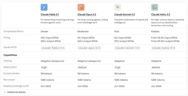
How large language models differ, and what to compare
Context window, reasoning effort, tool use, input types and price per token: how LLMs from Anthropic, OpenAI and Google differ, from their own pages.
Read the post
Where AI is heading: what the data shows and what is forecast
Where AI is heading, from dated reports: Stanford's AI Index, Epoch AI, METR and the IEA. What has been measured, what is forecast, and who said it.
Read the post
RAG explained: how retrieval works and when to use it
Retrieval augmented generation finds the right passages and puts them in the prompt. How it works, from the 2020 paper to vector search, and when to skip it.
Read the post